How does DASAPT calculate a 1D profile and its error bars?

This note compares a one-dimensional composition profile from commercial atom-probe software with the cylinder profile in DASAPT. The two curves describe the same idea: composition along a cylinder. They line up when the cylinder, the ranges, the ions in the denominator, and the distance origin are the same. Where they still differ, the cause is usually one of the choices below.

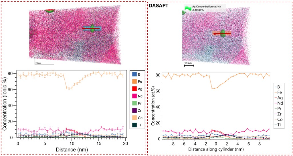
Left, commercial software: ionic percent, distance measured from one end (0 to about 20 nm), with error bars. Right, DASAPT: atomic percent along the cylinder, distance measured from the cylinder centre (about −9 to +9 nm). The Fe minimum sits near the middle of both axes. Shift the left-hand distance by about half the cylinder length and the two profiles meet.

左图是商业软件：离子百分比，距离从一端起算（大约 0 到 20 nm），带误差棒。右图是 DASAPT：沿圆柱的原子百分比，距离以圆柱中心为零（大约 −9 到 +9 nm）。Fe 的低谷都在轴的中部。把左图的距离平移大约半个圆柱长度，两条剖面对齐。

Which atoms are inside

The cylinder has a centre, a unit axis, a radius R, and a half-length H. For an atom at position r, the signed distance along the axis is s = (r − centre) · axis. The atom is kept when |s| ≤ H and its distance from the axis is at most R. Atoms removed by the current slice, cube clip, or ion-range filter are not counted.

The plotted distance is this same s. Zero is the centre of the cylinder, not one end. The first bin sits just after −H, and the last bin sits just before +H. The arrow drawn through the cylinder points toward increasing s. Reverse direction turns the axis by 180°, so the profile runs from the other end. A commercial proxigram that starts at 0 on an interface matches this axis after a shift of H, apart from the half-bin offset below.

Bins

The cylinder length is L = 2H. The number of bins is the length divided by the requested bin width, rounded to the nearest integer, and limited to 1500. The width actually used is then L divided by that integer, so the bins cover the cylinder exactly and can differ slightly from the number typed in the box. A request below 0.02 nm is raised to 0.02 nm. Bin b covers s from −H + bΔz to −H + (b+1)Δz, and the point is drawn at the centre of that interval. An atom exactly on the positive end is placed in the last bin.

Each ranged peak is counted on its own. For the ion curves, a trailing + or − is removed and the rest of the name is kept, so Fe+ and Fe2+ stay separate. Ions that hit no range go to Unranged. That series is omitted when the cylinder contains none.

Concentration

In a bin, n_i is the count of one species and N is the count used as the denominator. The atomic percent is 100 × C, with C = n_i / N.

In ion mode, N is the sum of the ions checked in Include in calculation. A species that is not included is left out of N and is also removed from Plot layers. Unranged enters N only when it is checked.

In element mode the same ion counts are split by formula. Digits at the start of an isotopic name are dropped. The charge, including the digit written before + or −, is dropped. TiO contributes one Ti and one O. Ti2O3 contributes two Ti and three O. n_i is the sum of those stoichiometric contributions, and N is the sum of the elements that are included. A bin with N = 0 is left blank.

Error bars

The concentration bars are the binomial standard error. The N counts in the bin are treated as independent draws, and each draw belongs to species i with probability C. The standard error of the fraction is

\[ \sigma_{C} = \sqrt{\dfrac{C(1-C)}{N}} \]

and the bar drawn in atomic percent is

\[ \sigma_{\mathrm{at.\%}} = 100\sqrt{\dfrac{C(1-C)}{N}} \]

with C = n_i / N. This is the value exported as atpct_err. The bar is shown on the concentration plot when Concentration error bars is checked. It is long when N is small. At 0% and at 100% the plug-in estimate is exactly 0, because a bin that is all one species, or none of it, has binomial variance zero under this formula.

A Poisson bar, 100 × sqrt(n_i) / N, is a different number. The binomial bar is that Poisson bar multiplied by sqrt(1 − C). At low concentration the two are close. Around 50 at.% the Poisson bar is about 1.4 times the binomial bar. The Poisson form does not fall to zero at 0% or 100%.

Counts use Poisson statistics: the standard error of a count n is sqrt(n). The density is the count divided by the slice volume pi R^2 dz, so its standard error is sqrt(n) divided by that volume. The volume is the full geometric slice for every bin. It does not shrink where the specimen fails to fill the cylinder, and the density falls there for that reason. The count and density plots do not draw these bars; the concentration plot is the one with the binomial bars.

Element mode puts the same binomial formula on the atom tallies. One molecular ion is still one detection: TiO adds two atoms to N from a single event. The bar treats those tallies as if they were the independent draws.

Delocalization

If Delocalization is larger than 0.01 nm, every count curve is smoothed before the percentages are formed. The Gaussian standard deviation is one third of the delocalization width. The kernel is cut at three standard deviations. Samples past either end of the profile are skipped and the kernel is not re-normalised there, so the two end bins lose some counts. After smoothing, neighbouring bins are correlated, and n_i and N need not be integers. The error bar still inserts those smoothed numbers into the binomial formula. It describes that smoothed bin, not the independent atoms before smoothing.

What to check when the two profiles disagree

• Distance origin. DASAPT uses the cylinder centre as zero and plots bin centres. A curve that starts at an interface needs a shift of H, and the half-bin centre can leave a shift of Δz/2.
• The denominator. Included ions, excluded ions, and Unranged change C even when the counts of one species match.
• Charge states. Ion mode keeps Fe+ and Fe2+ apart. Element mode adds them, and it splits molecules by stoichiometry.
• Smoothing. A non-zero delocalization moves counts between bins before the percentage and the error bar are computed.
• The error formula. A bar that stays open at 0% and 100%, or that is about 1.4 times longer near 50 at.%, is the Poisson form rather than the binomial form above.

中文

这篇比较的是商业原子探针软件里的一维成分曲线，和 DASAPT 圆柱剖面。两边都是沿一根圆柱看成分。圆柱、范围、分母里的离子、距离零点一致时，曲线应当重合。仍然分开时，原因一般是下面某一步的取法不同。

哪些原子算在圆柱里

圆柱由中心、单位轴向、半径 R 和半长 H 确定。原子位置是 r 时，沿轴的有符号距离是 s = (r − 中心) · 轴向。|s| ≤ H，并且离开轴线的距离不超过 R，这个原子才保留。当前切片、立方裁剪或离子序号过滤去掉的原子不计数。

图上的距离就是这个 s。零点在圆柱中心，不在某一端。第一格靠近 −H，最后一格靠近 +H。穿过圆柱的箭头指向 s 增大的方向。Reverse direction 把轴转 180°，剖面就从另一头算起。商业 proxigram 若把界面放在 0，把它沿距离平移 H 之后，才和这条轴对齐；另外还差下面说的半个分箱。

分箱

圆柱长度 L = 2H。箱数是长度除以设定的箱宽，四舍五入，并且不超过 1500。实际箱宽再用 L 除以这个整数，因此各箱刚好铺满圆柱，可能和输入的宽度略有差别。小于 0.02 nm 的请求会提到 0.02 nm。第 b 箱覆盖 −H + bΔz 到 −H + (b+1)Δz，点画在这一段的中心。正好落在正端面上的原子归进最后一箱。

每一个已标定的峰单独计数。离子曲线只去掉名字末尾的 + 或 −，所以 Fe+ 和 Fe2+ 仍然分开。没有落进任何范围的离子归到 Unranged。圆柱里一个都没有时，这一条不出现。

浓度

在一个箱里，n_i 是某一类的计数，N 是分母。原子百分比是 100 × C，C = n_i / N。

离子模式下，N 是 Include in calculation 里勾选离子的计数之和。没有勾上的种类不进分母，也会从 Plot layers 去掉。Unranged 只有被勾上时才进入 N。

元素模式把同一批离子计数按分子式拆开。同位素名字开头的数字去掉。电荷去掉，写在 + 或 − 前面的那个数字也去掉。TiO 贡献 1 个 Ti 和 1 个 O。Ti2O3 贡献 2 个 Ti 和 3 个 O。n_i 是这些化学计量贡献之和，N 是勾选元素的原子数之和。N = 0 的箱留空，不画误差棒。

误差棒

浓度误差棒是二项分布的标准误差。把该箱的 N 个计数看成独立抽样，每一份属于第 i 类的概率是 C。比例的标准误差是

\[ \sigma_{C} = \sqrt{\dfrac{C(1-C)}{N}} \]

画在原子百分比上的半高是

\[ \sigma_{\mathrm{at.\%}} = 100\sqrt{\dfrac{C(1-C)}{N}} \]

其中 C = n_i / N。导出的 atpct_err 就是这个数。浓度图上，勾选 Concentration error bars 才画出误差棒。N 越小，棒越长。在 0% 和 100%，这个插件估计恰好是 0：箱子里全是这一类，或完全没有这一类时，按该公式方差为零。

泊松式误差棒 100 × sqrt(n_i) / N 是另一个量。二项误差棒等于它再乘上 sqrt(1 − C)。低浓度时两者接近。50 at.% 附近，泊松式大约是二项误差棒的 1.4 倍。泊松式在 0% 和 100% 不会收到 0。

计数用泊松统计：计数 n 的标准误差是 sqrt(n)。密度是计数除以切片体积 pi R^2 dz，所以密度的标准误差是 sqrt(n) 再除以这个体积。每一箱都用完整的几何体积，样品没有填满圆柱时体积也不缩小，密度会因此下降。计数图和密度图不画这些棒；画出二项误差棒的是浓度图。

元素模式把同一个二项公式用在原子计数上。一个分子离子仍然只是一次探测：TiO 从一次事件往 N 里加了两个原子。误差棒把这些原子计数当作独立抽样来算。

Delocalization

Delocalization 大于 0.01 nm 时，先对每条计数曲线做高斯平滑，再算百分比。标准差取 Delocalization 宽度的三分之一，核在三倍标准差处截断。超出剖面两端的样本直接丢掉，端部的核不重新归一，所以两端的箱会少掉一部分计数。平滑之后相邻箱相关，n_i 和 N 也不一定还是整数。误差棒仍把平滑后的数代进二项公式。它描述的是平滑后的这一箱，不是平滑前那一组独立原子。

两条曲线对不齐时先看这些

• 距离零点。DASAPT 以圆柱中心为零，并且画在箱中心。从界面起算的曲线要平移 H，半个箱宽还会留下 Δz/2 的错位。
• 分母。勾选哪些离子、是否包含 Unranged，都会改变 C，即使某一类的计数相同。
• 电荷态。离子模式把 Fe+ 和 Fe2+ 分开。元素模式把它们加在一起，并把分子按化学计量拆开。
• 平滑。Delocalization 不为零时，百分比和误差棒用的是平滑之后的计数。
• 误差公式。在 0% 和 100% 仍然张开，或在 50 at.% 附近大约是二项误差棒 1.4 倍的，是泊松式，不是上面的二项式。